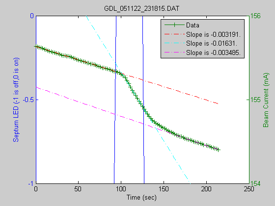
Mike Forster 2005.11.28
[file,path] = uigetfile...
    ('C:\MATLAB7\work\MachineStudies\LifetimeMeas\gdlData\*.dat');
pathfile = [path file];
fid = fopen(pathfile,'r'); % Open text file
while (~feof(fid))

    % Read preamble data:
    PreambleText=textscan(fid,'%s %[^\n]',6);

    % Read data
    FormatString='%s %n %n %n';

    InputData=textscan(fid,FormatString);

end
fclose(fid);
times = InputData{1,1};
dtimes = datenum(times(:),'yymmdd_HHMMSS');
t6 = datevec(dtimes(:));
tbase = t6(1,:);
t = [];
for ti = 1:(size(t6))(1);
    t(ti) = etime(t6(ti,1:6),tbase);
end;
t = t';
onoff = InputData{1,2};
cmd = InputData{1,3};
bcur = InputData{1,4};
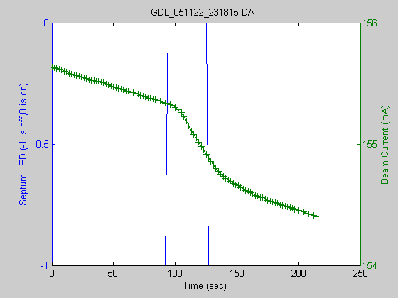
Plot graph with 2 y-axes Returns two axes objects (AX(1) and AX(2)) and two graphics handles (H1 and H2)
figure;
[AX,H1,H2] = plotyy(t,onoff,t,bcur,'plot');

% Add markers to the beam current data
set(H2,'Marker','+');

% set y axes labels
set(get(AX(1),'Ylabel'),'String','Septum LED (-1 is off,0 is on)');
set(get(AX(2),'Ylabel'),'String','Beam Current (mA)');

% set x axis label
xlabel('Time (sec)');

% Set title to file name
% set Interpreter to None so _ are shown correctly
title(file,'Interpreter','None');
offindices = find(onoff == -1);
onindices = find(onoff == 0);
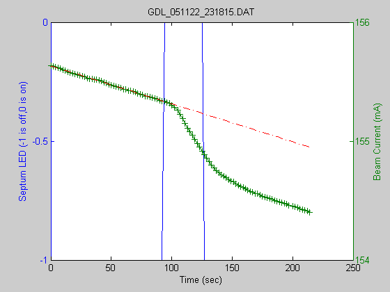
beginning to septum turned on => onindices(1) set up y = Ax equation to solve using least squares
y = bcur(1:onindices(1));
tregion = t(1:onindices(1));
A = [ones(size(tregion)) tregion];
x = A\y;
slope(1) = x(2);
axes(AX(2));
hold on;
A = [ones(size(t)) t];
plot(t,A*x,'r-.');
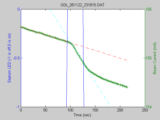
middle of septum turned on => round(median(onindices)) to septum turned off set up y = Ax equation to solve using least squares
midind = round(median(onindices));
y = bcur(midind:onindices(end));
tregion = t(midind:onindices(end));
A = [ones(size(tregion)) tregion];
x = A\y;
slope(2) = x(2);
A = [ones(size(t)) t];
plot(t,A*x,'c-.');
middle of last region => round((onindices(end)+offindices(end))/2.0) to septum turned off => offindices(end) set up y = Ax equation to solve using least squares
midind = round((onindices(end)+offindices(end))/2.0);
y = bcur(midind:offindices(end));
tregion = t(midind:offindices(end));
A = [ones(size(tregion)) tregion];
x = A\y;
slope(3) = x(2);
A = [ones(size(t)) t];
plot(t,A*x,'m-.');

legend('Data',sprintf('Slope is %0.4g.',slope(1)),...
    sprintf('Slope is %0.4g.',slope(2)),...
    sprintf('Slope is %0.4g.',slope(3)));
legend show;

hold off;
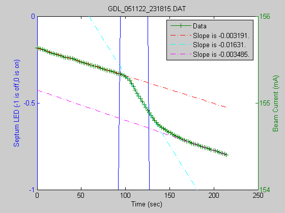
use regexp to get rid of file extension
outfile = regexprep(pathfile,'\.dat','','ignorecase');
% print needs to be called in the following format
% in order to pass a variable as a file target
pause;
print('-dpng','-r80',outfile);