2009.08.11 - Vertical dispersion studies

Ideal Lattice (eta_y = 0)

Motivation: For CesrTA, we wish to achieve an RMS vertical dispersion (eta_y) of less than 1cm. Factors that can affect our dispersion measurement include single-channel gain errors on the BPM buttons and tilts of the BPMs. How well must we know the BPM tilts and gain errors in order to achieve a measurement accurate to within 1cm RMS?

Start by simulating an ideal lattice (actual eta_y = 0), and "measure" the vertical dispersion by varying \delta E such that it corresponds to a frequency change of +/-5kHz. (\delta E / E = +/-0.00148). Begin introducing BPM tilts, gain errors and resolution (in that order) in the following way:

• For BPM tilts, use a simple rotation matrix
• For gain errors and resolution, convert each (x,y) to four button signals b_i. Introduce random (Gaussian) gain errors on each of the four b_i's. Resolution is simulated as an additive uncertainty in the signal. The overall "measured" button value is therefore: b_i' = g_i * b_i + \delta b.
• Resolution is determined by: "measure" position (1mm,1mm) and convert to four b_i's. Remeasure (1mm+1\sigma,1mm+1\sigma), and consider the average change in button signals for b1 and b4. Use this as the additive uncertainty in button signals.

Repeat the initial \eta_y simulation, but introduce errors at the following levels:

• BPM tilts: [0,10, 15, 20, 25, 30, 35] mrad
• Gain errors: [0.,0.01,0.02,0.05,0.07,0.10,0.15,0.20,0.5,1.,5.,10.,15.,20.] percent
• Resolution: [0.,10.,20.,35.] microns

For each combination of BPM tilt, gain error, and resolution, find the RMS vertical dispersion "measured". Repeat the simulation for 100 random seeds and average the resulting RMS values.

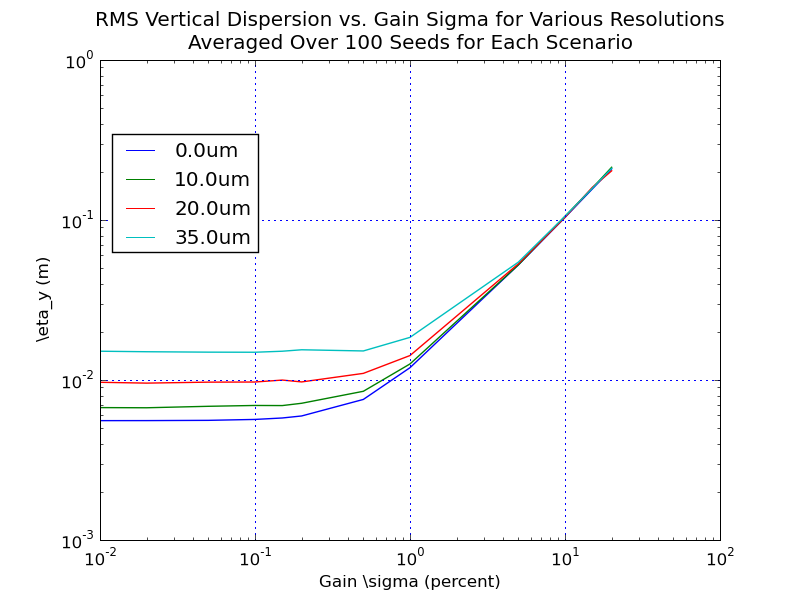
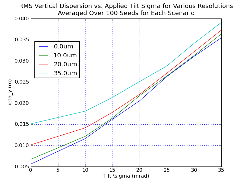
Now plot cross-sections of the results. First consider if we set either BPM tilts or gain errors to zero, and vary the other parameter for different resolutions:

Note the different scales for the two plots. A few observations:

• For small gain errors (sigma < 0.6%), eta_y is resolution dominated. Larger gain errors quickly dominate. This is expected.
• For the range of tilts examined, BPM tilts seem to dominate eta_y after about 10-15mrad. This is again not surprising.
• If we consider our target of knowing the vertical dispersion to within 1cm, then a 35-micron resolution already prevents us from reaching our goal. For a 10-micron resolution, we have a tolerance of either 0.6% gain errors or ~6mrad BPM tilts.

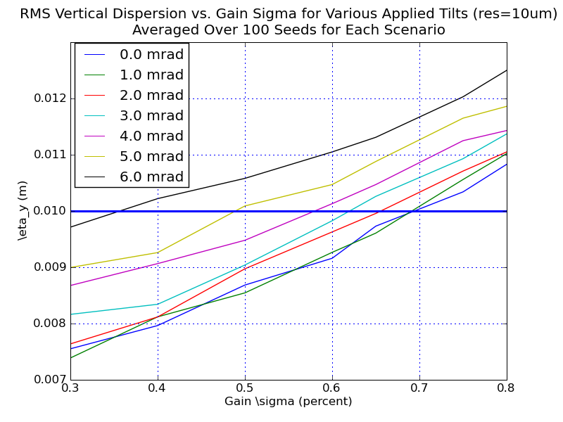
What happens if we fix the resolution and consider the "cross terms", i.e., applying both gain and tilt errors? The plots below show eta_y vs. gain sigma, for various BPM tilts, at a fixed resolution. Left shows 10um resolution, right is 35um:

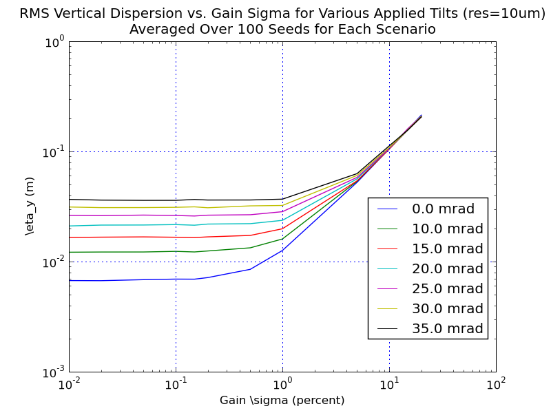
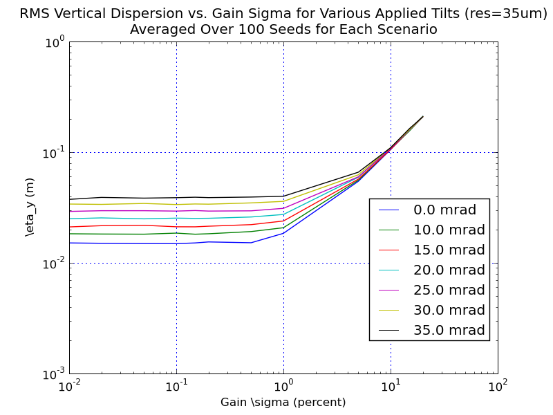
As before, each scenario is repeated and averaged over 100 random seeds. A few observations:

• Once again note that at 35 microns, we are already above the 1cm target.
• For 10 micron resolution, we can tolerate somwhere between 0-10mrad BPM tilts.

Recall the "actual" eta_y is zero here-- this is an "observed" disperison that doesn't actually exist. We can then plot the combinations of misalignments where we achieve an RMS of 1cm observed eta_y.

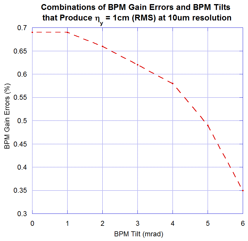
We can interpret this plot as a "tolerance range": that is, anything below this curve is a tolerable combination of misalignments that will yield a measurement within 1cm (RMS) at a 10um resolution. It is not possible to achieve 1cm RMS eta_y with a 35um resolution.

Simulating January 2009 Results:

Motivation: In January 2009 we achieved a measured RMS eta_y of ~2.5cm. However, the measured beamsize corresponded to an RMS eta_y of roughly 1.4cm. Contributions to the beamsize from coupling are taken as negligible. What combination of BPM tilts and gain errors would make an actual 1.4cm RMS vertical dispersion look like 2.5cm?

Start by taking the ideal (eta_y = 0) lattice and introducing vertical dispersion. Use steering V10W to generate 1.4cm RMS eta_y. Apply tilts and gain errors in the same fashion as before, repeating each scenario for 100 seeds and averaging the results. Only consider the 35um resolution scenario, since this is what we believe our present limit to be.

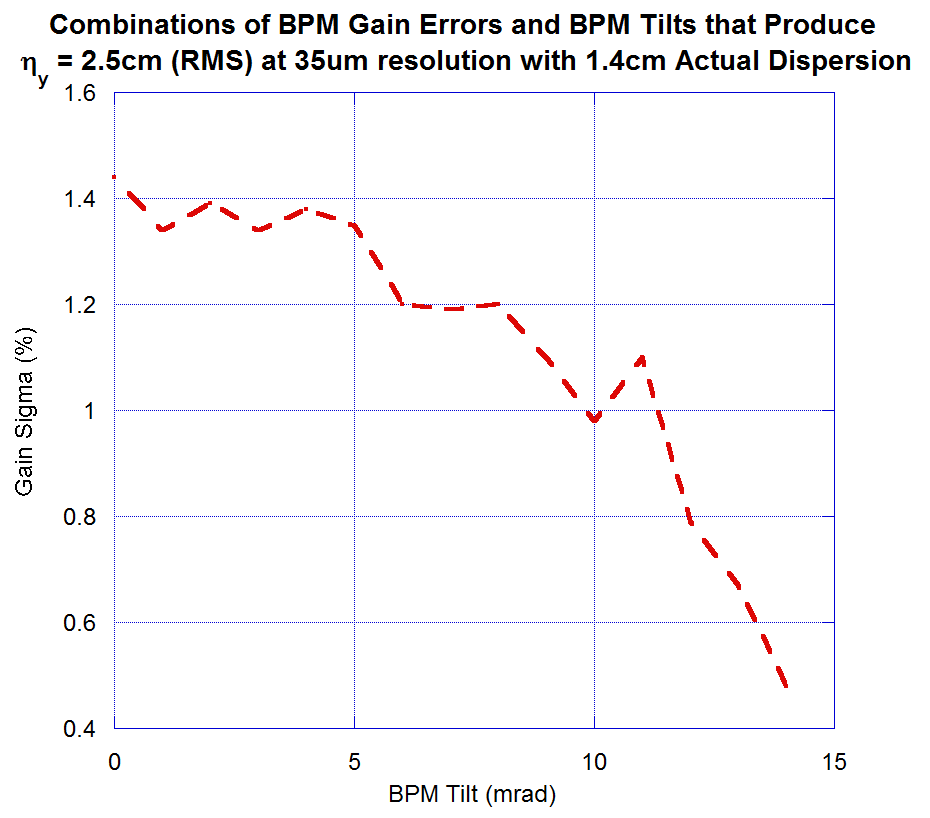
Note that there are more data points in this curve than the previous plot. This may contribute to why it looks less smooth. Again, we can interpret this plot as describing the parameter space that would account for our measurements in January.

From ORM studies, we believe our tilts to be around RMS ~ 35mrad, and from preliminary results of BPM gain mapping we think our gain errors are on order of ~ 10%. This would put us well outside the range of parameters that would produce the measured eta_y from January. However, Jim Sexton's survey results suggest an RMS BPM tilt on order of ~6mrad, which would be well within the range of this plot. This would suggest our BPM gain uncertainties are below roughly 1.2% RMS.