Introduction
fa — the fraction of events that are smeared according to the second Gaussian. We'd like to see this parameter's effect on the fitting procedure by looking at its corresponding log likelihood value.
Procedure
Mode 0 (Kpi)
- For mode 0 (Kpi), to plot the fa vs. log likelihood for data, we get1:
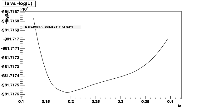
The central value of fa from Signal MC table is: 0.182, we can read
the -Log(L) value from the plot as: -981717.57. By reducing the
maximum value of Log(L) by 0.5, i.e. -981717.07, we have the
corresponding fa to be 0.13 and 0.38 respectively.
Then we fit the data with 0.13 and 0.38, comparing the yields with the regular one.
- fa 0.13
| Mode | data diff(%) | signal diff(%) | generic diff(%) |
|---|---|---|---|
| D0 &rarr K- &pi+ | 0.01 | 0.01 | 0.05 |
| D 0&rarr K+ &pi- | 0.01 | 0.01 | 0.03 |
- fa 0.38
| Mode | data diff(%) | signal diff(%) | generic diff(%) |
|---|---|---|---|
| D0 &rarr K- &pi+ | -0.14 | -0.04 | -0.11 |
| D 0&rarr K+ &pi- | -0.15 | -0.04 | -0.09 |
Mode 1 (Kpipi0)
- For mode 1 (Kpipi0), we get2:
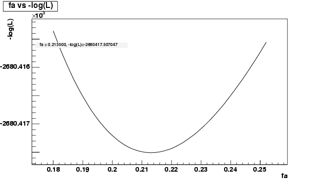
The central value of fa from Signal MC is: 0.196,By reducing the
maximum value of Log(L) by 0.5, we have the corresponding fa to be
0.19 and 0.24 respectively.
Then we fit the data with 0.19 and 0.24, comparing the yields with the regular one.
- fa 0.19
| Mode | data diff(%) | signal diff(%) | generic diff(%) |
|---|---|---|---|
| D0 &rarr K- &pi+ &pi0 | -0.01 | 0.01 | 0.00 |
| D 0&rarr K+ &pi- &pi0 | -0.01 | 0.01 | -0.01 |
- fa 0.24
| Mode | data diff(%) | signal diff(%) | generic diff(%) |
|---|---|---|---|
| D0 &rarr K- &pi+ &pi0 | 0.03 | -0.09 | -0.05 |
| D 0&rarr K+ &pi- &pi0 | 0.03 | -0.09 | -0.05 |
Conclusion
The difference are below 0.15% level, negligible.