a fit2d SAXS/WAXS primer

Detlef Smilgies, CHESS D1 station

version 2/27/2007

INDEX

final remark

disclaimer

fit2d is a free program running on LINUX and MS Windows and can be downloaded from ESRF. Check out the fit2d homepage for terms and the latest version. Click here for the fit2d on-line manual; an introduction can be found here. For use of the advanced fit2d features please include an acknowledgement.

This fit2d primer is meant for the SAXS/WAXS users at CHESS D1 station. My very incomplete list of fit2d features are some things that work for me and come up all the time. fit2d has a 300 page plus manual that can be viewed on-line or downloaded from ESRF - please take a look to find out about further details. I'll be glad for feedback on this primer and to learn new tricks - but don't ask me any detailed fit2d questions: this primer sums up pretty much what I know and use of fit2d.

No ready-made program will take care of all fine details of the analysis by itself. For instance proper Lorentz and polarization factor corrections depend on the experiment. So if you are very picky, the best way is to do this part yourself. This is particularly true for GISAXS and GIWAXS data, for which there are still some open questions about proper data processing.

A final hint: The way the various items are ordered roughly corresponds to their difficulty. If you are unfamiliar with fit2d, it may make sense to go through the list in order. Right-click here and choose "save target as" to download the datafile I used in the examples below.

start-up

The easiest way of working with fit2d is, if you start it from the data directory, which thus becomes the default input directory. Open a new LINUX window, go to your data directory (cd /[USER]/corr) and type fit2d at the LINUX prompt to do so. I usually devote desktop 2 for fit2d, to keep desktop 1 clean for spec.
fit2d needs to reserve some initial memory space for reading in images. For the MedOptics detector I recommend to use 1200 by 1200 as initial array size.
Use memory arrays (answer YES) for speedy data handling, don't use variance arrays (answer NO).
Click O.K which gets you to the fit2d main menu.

display an image

goto SAXS/GISAXS > input
find the data directory and choose an image file (extension .tif); when fit2d gets started in the data directory, you are already there
default false colors are quite nice - see manual for other choices
set the scale: SAXS/GISAXS > Z-SCALING; choose "LOG SCALE" and set "USER MIN/MAX" to 1 and 15000: these are the default values to check whether the detector is happy - white regions indicate that the exposure was too long
get back to SAXS/GISAXS menu by hitting EXIT; this will be the default in many menus and I won't mention it again
use SAXS/GISAXS > ZOOM IN to zoom into a region
use SAXS/GISAXS > DISPLAY > SLICE to make a 1D cut through the image

Figure 1. Raw WAXS data of MedOptics CCD camera: silver behenate calibration sample (10 keV photons, sample detector distance about 100mm).

display a series of images

go to main > FILE SERIES > COMPOSITE
input first and last file and FILE INCREMENT (for instance increment2 reads in every other file)
SUBTRACT: NO
ROI: optionally YES or NO
NO. PER ROW: aim for square arrays for best quality; if some images are missing to fill the array, empty images are given in black
RE-BIN NO.: the image size for a composite image gets too large, if the resolution is not reduced. Increase suggested binning by 1, since fit2d tends to overestimate the size of available memory which can crash the program

notes:

only files with identical names other than the file number can be combined into a series (otherwise make renamed copies of the files)
this feature is very useful to create an overview of all data

background subtraction

for very weak scatterers or strongly scattering sample environments such as x-ray capillaries or liquid cells it may be important to take background images, in order to subtract out the sample cell scatter. This can be done in the IMAGE PROCESSING menu:

read in background image: INPUT
click EXCHANGE
read in data image: INPUT
click MATH > SCALED SUB: scaled subtraction allows finetuning a background scaling parameter
finetune scalefactor
you can save the background-subtracted image using OUTPUT to create a file in tiff format for further processing

calibrated plots

direct beam

first task is always to find the direct beam mark (through an attenuator!). I usually make sure that at least one set of calibration data is collected for each detector configuration. Such files are typically called "AgBeh-xxxxx".
go to SAXS/GISAXS > BEAM CENTRE > 2D GAUSSIAN FIT and click on the beam mark
the program will remember this position, unless a new beam center calibration is performed; fit results are provided on the fit2d ASCII window

distance/wavelength calibration

Usually I know the x-ray wavelength to within 1% from the mono calibration (checked at each beginning of a run)
The sample/detector distance is harder to get this accurate, in particular for WAXS
I use a Ag behenate standard (d-spacing d=58.38 A); some people also use Ag stearate (d=47.??A).
fit a pronounced powder ring - goto SAXS/GISAXS > BEAM CENTRE > CIRCLE COORDINATES and fit a behenate powder ring (follow instructions)
read the radius value R in pixels from the ASCII screen; depending on which ring you chose (number n) the corresponding d-spacing is d/n
For SAXS, where all is linear, you can convert directly from pixels to Q-space using R. For WAXS the non-linearity of Bragg's law is starting to show and some cross checks may be useful. However, the data range does not extend far enough to get a good fit of both distance and wavelength, as can be done in powder diffraction (you can try the POWDER DIFFRACTION menu instead of SAXS/GISAXS; let me know, if you can get the calibration feature to work)

azimuthal integration

for SAXS/WAXS from non-textured samples you want to simply integrate the intensity rings and create a simple radial plot:

go to SAXS/GISAXS > INTEGRATE
integration needs a fair amount of input data, however, these will be saved, and can be recalled for the next image to be analyzed
the important input parameters are:

pixel size: 47.19 microns for the MedOptics detector in both directions
sample to detector distance L: calculate from behenate ring radius R: L(mm)=R(mm)/tan[2•asin(n•λ/2•d)] and n ist the order of the behenate ring used
wavelength λ: will be provided by me
the direct beam coordinates were already determined in the previous step

You have a choice of plot axes:

scattering vector Q (inverse nm)
scattering angle 2theta (deg)
d-spacing (Angstroem)

There are some other parameters that are related to the rescaling of the intensity, which however, depend on the scattering geometry and I have some reservations to use some of the fit2d features:

CONSERVE INT. : NO is recommended in combination with other fit2d features
POLARIZATION : does not explain whether it is s- or p-polarization, so if I really care, I choose NO and do it myself. This factor does not have effect on SAXS, and also for WAXS from organics, scattering angles are still smaller than 20 deg with the MedOptics camera, so this correction is not very important either.
GEOMETRY COR. take care of the transformation from a planar area detector to angle space (for math freaks: it's the Jacobian), so this one I use: YES

Some processing parameters:

MAX. ANGLE: I use the default suggested by fit2d
SCAN BINS: a value of about 1000 yields good-looking curves
MAX. D-SPACING: depends on your sample:

for WAXS, 100 Å is a good start
for SAXS, 2000 Å will do for all D1 can resolve

Final remarks:

You only have to set-up all of these parameters once, and the you can go through your hundreds of images, provided the scattering geometry remained the same
You can save the numeric output data using SAXS/GISAXS > OUTPUT and choose option CHIPLOT for further analysis with your own favorite software. The default values in the CHIPLOT menu will result in an ASCII file with a small header and the plot values written as an x and a y column of values (don't try to understand the settings). You can choose/modify the filename using the FILE NAME option.
You can save any plots using SAXS/GISAXS > PRINT; the plot is written to a postscript file.
Before you INPUT the next file to process, use EXCHANGE to get the program into the right mode. This is important in the SAXS/GISAXS menu, some of the other menus are more forgiving.

Reference: A P Hammersley, S O Svensson, M Hanfland, A N Fitch, and D Häusermann, ``Two-Dimensional Detector Software: From Real Detector to Idealised Image or Two-Theta Scan'', High Pressure Research, 14, pp235-248, (1996)

(projections)

PROJECTION : Integrate rectangular region to 1-D scan. This uses the beam centre and a user input coordinate to define an integration line. A second user input coordinate defines the width of the integration region. Pixels within this region are effectively ``collapsed'' onto the integration line, and then re-binned to the required 1-D output scan. This type of integration is specifically for grazing incidence data. (cited from fit2d on-line manual - I still have some question about how this feature exactly works)

1D peak fitting of calibrated data

before you get started, the Z-SCALING mode has to be set to LINEAR (in any menu you happen to be in). In order to make data visible again, if you come from LOGARITHMIC, use FULLY AUTOMATIC or WEAK PEAKS. These features work for the LINEAR scale, but yield poor scaling in the LOG scale.
goto MAIN > MFIT > INITIALIZE
provide rough starting parameter:

use POLYNOMINAL for the background; a polynom of 6th order works for me
choose model for peaks (GAUSSIAN, etc.) and follow instructions
provide starting values for each peak
starting curves are shown that should look reasonable
EXIT

OPTIMISE should give you a nice fit
RESULTS displays the fit parameters in your chosen calibrated coordinates which can be saved to a file using SAVE
ASCII OUTPUT can be optained using CHIPLOT (to be tested)
PRINT the output, if you want to use the graphics (see "calibrated 2D plots")

Figure 2. Integration of AgBeh raw input data and succesive fit (6th order polynominal background and 7 Gaussians; the 2 small peaks on the right were not attempted to be fitted). The bottom plot shows the residuals.

Reference: A P Hammersley and C Riekel, ``MFIT: Multiple Spectra Fitting Program'', Synchrotron Rad. News, 2, pp24-26, (1989) .

cake plots

for textured samples, i.e. if powder rings have structure or for partial powder rings, you may want to fit the angular width of these features. Here the CAKE menu comes handy: CAKE converts the x,y image to a calibrated polar plot, where the x axis can be 2-Theta (deg), q (inverse nm), or d (Å), and the y axis is the azimuth angle around the beam
so cake yields another 2D image, which however is very suitable to determine angular widths
linescans via DISPLAY > SLICE show the texture of the rings
in lieu of a more elegant method I usually OUTPUT the linescan to a spreadsheet for further fitting (Origin, Excel, etc.)

CAKE uses the same parameters as INTEGRATE (see above); additionally you have to indicate

START AZIMUTH: choose in first quadrant for a continuous output angular range
END AZIMUTH: go in counter-clockwise direction from start azimuth
INNER RADIUS: can be as small as the direct beam position
OUTER RADIUS: can be as far out as the image extends
note: the CAKE plot will always provide a 360 deg range starting from the MINIMUM AZIMUTH and going in counter-clockwise direction.

some conversion parameters:

1 DEG AZ : YES if 360 steps yields decent output, NO - for a finer grid (e.g. 720)
AZIMUTH BINS: go in multiples of 360 for interpretation (see below)
RADIAL BINS: 500-1000 looks good
note: for this transformation you will appreciate how lightning-fast fit2d cranks through the data - try the same in Origin!
note: the usual fit2d features seem to have some problem with the transformed plot. In particular the pixel size does not come out right. However, choosing 1 DEG AZ. : YES, or similar, provides a simple angular bin size (of 1 deg) for further processing. Ideally slices or projections (integration of intensity over a range onto a line) could be used to determine angular width.

Other parameters

some other parameters as explained in INTEGRATE above
after the transformation, go to ASPECT RATIO and choose NO for a full size plot
for printing or writing the CAKE plot to a spreadsheet see below.

Figure 3. Sample output from CAKE: Shown are the silver behenate rings from the raw image converted to a azimuth-versus-Q_radial plot. The powder rings are homogeneous showing the high quality of the conversion. For a textured sample powder ring features can be fitted to measure angular features.

Special option: Integrations with CAKE

To make the example more meaningful, I will demonstrate the CAKE integration features with a more meaningful example. Poly(hexyl thiophene) (P3HT) is a common semiconducting polymer. The side-chains order the polymer backbone in lamellae parallel to a silicon wafer surface. Polymer backbones are closely packed due to pi-stacking of the monomer aromatic rings. The degree of order depends on details of the preparation conditions, and is subject to current studies.

Figure 4. GIWAXS from a poly(hexyl thiophene) film spin coated onto a silicon wafer covered with the native oxide.
Incident angle was chosen as 0.3°. I thank Satoyuki Nomura and George Malliaras for providing a sample.

Two CAKE special options are of immediate interest:

By setting azimuthal bins to 1, a single 1-D radial 2-Theta or Q-space scan can be obtained which is integrated over a sector whose angular width is given by the azimuth parameters. This way the integration region and the signal-to-noise ratio can be better controlled and problematic regions (edges, bad spots) can be better avoided than using INTEGRATE.


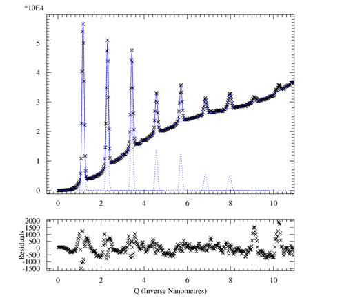
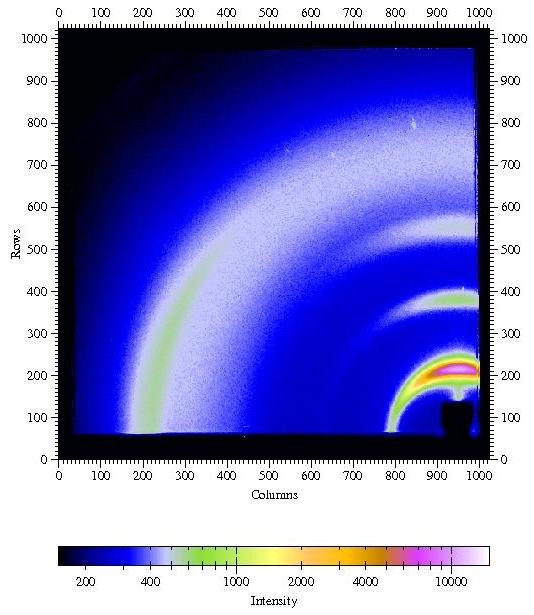
Fig 5a: Radial scan (90-890 pixels in 800 steps), integrated over azimuth range of 90°-120°. The (00L) reflections indicative of lamellae formed by the ordering of the alkyl side-chains show up prodominantly in the perpendicular direction, i.e. the lamellae are parallel to the surface. The broad powder ring is due to the amorphous silicon oxide layer at the wafer surface.	Fig 5b. Radial scan (90-890 pixels in 800 steps), integrated over azimuth range of 120°-180°. In the in-plane direction the (100) peak due to the pi-stacking of the aromatic rings of the polymer back-bone can be found, i.e. polymer chains are parallel to the surface and parallel to each other. Weak (00L) powderrings indicate that the lamellae are not perfectly parallel to the substrate.

(001)

(002)

(003)

silicon oxide powder ring

(001) powder ring

(002) powder ring

(100) (pi-stacking)

silicon oxide powder ring

By setting the number of radial bins to 1, and selecting the ''cake'' as an sector with specific radial vales, an integration of intensity versus azimuth may be obtained. This is very useful for texture analysis. In the P3HT case, the azimuthal width characterizes, how parallel the P3HT lamellae are with regard to the substrate.

(a)

(b)

(c)

(d)

Fig 6. Azimuthal scans fron 90 to 180 in steps of 1 for the four reflections identified above. A narrow radial range was chosen around each arc of intensity: (a) 90-250 pixels for the (001) reflection, (b) 250-400 pixels for (002), (c) 450-540 for (003), and (d) 680-790 pixels for the (100) reflections. Azimuthal widths are comparable. Note that (100) is in the perpendicular direction of the (00L) reflections and the its background is higher, as (100) is located on top of the broad powder ring of the amorphous silicon oxide layer.

For further analysis the azimuth distributions can be fitted as shown above. For writing the distributions to an ASCII file for creating publishable figures, use OUTPUT > CHIPLOT.

Tricks & Traps - Some things I found the hard way

before you INPUT the next image, hit EXCHANGE: this recalls the previous 2D data image settings (and the detector pixel size before the transform !!).
If you forget to EXCHANGE, chack INTEGRATION parameters carefully, and fix whatever looks wrong - in particular pixel sizes, and radial range.
use REMEMBER ROI to save your integration region - the you will get the same region each time in a file series: you can skip START AZIMUTH etc. and directly proceed to INTEGRATE. By default this feature is enabled on fit2d start-up.
At times I have gotten stuck in CAKE beyond rescue - in the worst cake close fit2d and restart from scratch.

calibrated 2D plots

I have not yet been able to find a feature in fit2d that handles this task in an elegant way, i.e. converting from x, y (pixels) to q_x, q_y (inverse Angstroem).

Here's the brute force way which is only good for SAXS or GISAXS maps, when the coordinate transformations are linear:

determine the (q_x_min, q_y_min) values of the left bottom corner point of the image from the beam center and Ag behenate calibration
determine the stepsize per pixel q_x_step and q_y_step
generate a plot using commands from above, then rescale the plot axes to these values:

go to the keyboard interface: MAIN > KEYBOARD
now typ the following command on the ASCII screen which will prompt you for the four values determined above: AXES SCALES > q_x_min, q_x_step, q_y_min, q_y_step
switch back to graphical interface: IMAGE; this has to be done after each step for changes to take effect on the image
other useful commands to generate publication-grade figures include

remove default labels: SET X-LABEL STYLE > no; SET Y-LABEL STYLE > no
make numbers larger: SET ENUMERATION STYLE ; in menu choose color BLACK and size 2
define major ticks: SET TICK POSITIONS
define minor ticks: SET AXES STYLE
define user region of image: REGION
high quality output: PUBLICATION QUALITY
for more detailed information see reference manual

if a series of images is to be reformatted, it is worth while to learn how to write a fit2d macro

PRINT to postscript file
a program like ghostview (available free on the internet) can reformat the postscript to a graphics file format like png or jpeg for use in publications
unfortunately 1D slices from the rescaled plot do not conserve the calibration and are plotted in relative pixel units
calibrated projections onto a line can be obtained using PROJECTION. Please check the fit2d manual for details (I still have to work this out).

See also Peter Busch's fit2d notes.

For D1-style GIWAXS, the non-linear coordinate transformation form pixels to scattering angles to q-components has to be done with another program, for instance an Origin 7.0 spreadsheet.

final remark

This page is still in development, but is meant to provide the backbone for on-line data analysis at CHESS D1 station. Please report errors to me. If you find another useful fit2d feature to include, let me know. DS